| States: Suppose we have some system which we are observing. We simplify all of the complication of the system and just classify it, every time we look at it, as being in one of a finite number of states, $S_1,\dots,S_n$. |
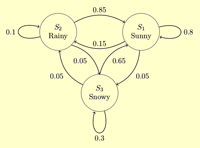
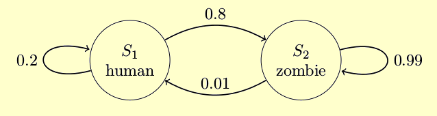
A1) An example might be the weather, which we think of as being Sunny, Rainy, or Snowy, which would be the states $S_1$, $S_2$, and $S_3$, respectively.B1) Another example might be a person ... during the time of the zombie apocalypse, whom we would classify as being human or zombie, being the states $S_1$ and $S_2$.
| Time: Next, let us suppose we observe the state of the system only at certain specific moments in time, every time some clock ticks. |
For the final assumption of this model, we will imagine the system moving
merrily on its way, transitioning from state to state at every tick of the
clock. Let us suppose there could be some randomness in the transitions
— they are only probabilistic — but these probabilities satisfy
| The Markov Hypothesis: The probabilities that the system, when in state $S_i$, will transition to state $S_j$, depend only upon the current state $S_i$. |
Note: if you are not too comfortable with probability calculations, just think of the probabilities we will use as fractions of the time that something happens. So if we say that the probability of going from state $S_1$ to $S_2$ is $.17$, just think of that as saying that about 17% of the time when the system is in $S_1$, it will go to $S_2$ at the next clock tick. Equivalently, think that in your database of observations of the system, out of 100 times it was in $S_1$, 17 times the next state was $S_2$. [This is what is called the "frequentist" philosophy of probability, which stands in opposition to the "Bayesian" approach.]
Note one consistency condition on these diagrams: every time the system is in some state and the clock ticks, it goes to some next state (possibly the one it was already in). That means that the sum of the labels on all of the arrows leaving each state blob must be one!
A2) The state diagram for weather in Pueblo, using the weather states mentioned above, might look like:B2) In a zombie apocalypse scenario where some small number of zombies get cured, the state diagram might look like: Note that what this is saying is that any given human has about an 80% chance of being bitten by a zombie, and thus becoming a zombie, and a 20% chance of avoiding that bite, each day (if the clock ticks in this model are days). Zombies, on the other hand, mostly just wander around staying zombies, except for 1% chance they have of being lucky enough to spontaneously cure on any given day.
| Definition: The transition matrix $T$ of a Markov model is the $n\times n$ matrix whose $(i,j)$ location $t_{ij}$ is the probability of the system transitioning from state $S_j$ to state $S_i$. |
A3) The transition matrix coming from the above state diagram for weather in Pueblo is $$ \begin{pmatrix} .8&.85&.65\\.15&.1&.05\\.05&.05&.3 \end{pmatrix}\quad . $$ B3) The transition matrix for the above zombie apocalypse scenario is: $$ \begin{pmatrix} .2&.01\\.8&.99 \end{pmatrix}\quad . $$
The way we have organized the transition matrix, the $j^{\rm th}$ column corresponds to all the probabilities for transition from $S_j$ to any state. As we observed above, these must total $1$ — the system transitions from $S_j$ to some state, after all! That means that all Markov transition matrices are examples of the following:
| Definition: A square matrix is said to be stochastic if all of its entries are non-negative and the sum of the entries in the any column is $1$. |
[The following approach with populations is the best way to talk about things in the "frequentist" point of view.]
Suppose now we have a large number, maybe $N$, of copies of our Markov system, all working in parallel and independently. We will describe the configuration of which states each copy is in by
| Definition: A state vector for $N$ parallel copies of an $n$-state Markov system is a column vector $\vec{s}\in\RR^n$ whose $i^{\rm th}$ entry is the number of copies of the system which are in state $i$. |
B4) In the above zombie apocalypse scenario, suppose a small town has $1000$ human inhabitants and $1$ zombie. The state vector would be $\vec{s}=\begin{pmatrix}1000\\1\end{pmatrix}$.
Well, there are $s_1$ system copies in state $S_1$. Of these, a fraction of size $t_{11}$ will stay in state $S_1$, yielding $t_{11}s_1$ copies in $S_1$ after the tick.
There are also $s_2$ copies in state $S_2$ before the tick, of which a fraction of size $t_{12}$ will transition to state $S_1$. This provides an additional $t_{12}s_2$ copies in state $S_1$ after the tick.
Proceeding in this way down each of the current states of the system copies, we end up with a total of $t_{11}s_1+\dots+t_{1n}s_n$ copies in state $S_1$ after the tick.
Exactly the same reasoning says that after the clock tick, there will be exactly $t_{i1}s_1+\dots+t_{in}s_n$ copies in state $S_i$.
Putting all of these formulæ into a vector and remembering what matrix multiplication looks like, we get the following expression for the state vector $\vec{s}^\prime$ after the clock tick: $$ \vec{s}^\prime = \begin{pmatrix}t_{11}s_1+\dots+t_{1n}s_n\\ \vdots\\ t_{n1}s_1+\dots+t_{nn}s_n\end{pmatrix} = T\vec{s}\quad . $$ In other words
| Transitioning: Each tick of the clock, the state vector $\vec{s}$ of a collection of $N$ parallel Markov systems is changed by multiplication on the left with the transition matrix $T$ of the system. As a consequence, the state vector after $k$ ticks of the clock will be $T^k\vec{s}$. |
| Definition: A steady state vector [also called stable distribution] of a population of $N$ parallel Markov systems is a state vector $\vec{s}$ with the property that $T\vec{s}=\vec{s}$, where $T$ is the transition matrix of the Markov systems. |
One thing that, with our training in this Math 207 class, we should immediately notice, is:
| Theorem: A steady state vector of a population of $N$ parallel Markov systems, each having transition matrix $T$, is an eigenvector of $T$ with eigenvalue $1$ and whose entries are all non-negative and sum to $N$. |
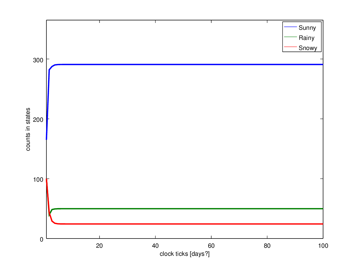
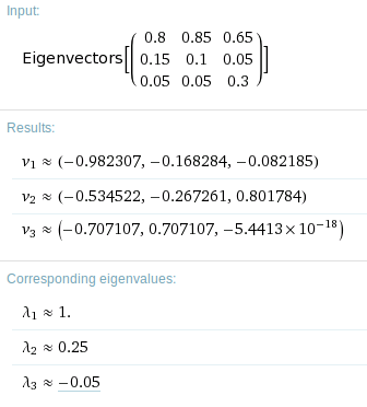
A4) Imagine taking $365$ random days of weather in Pueblo and running them forward in time according to the weather model given above until they reach the stable distribution. That distribution will tell us how many Sunny, Rainy, and Snowy days there will be in a "typical" year in Pueblo (by this model). We can find that by starting with the state vector $\vec{s}=\begin{pmatrix}165\\100\\100\end{pmatrix}$ and running it forward many clock ticks, say 100. This is a graph of the numbers of days in each state over those 100 ticks:The first eigenvector it computed corresponds to the first eigenvalue, $\lambda=1$. Unfortunately, it is not non-negative and having sum of 365! But all of its entries are at least of the same sign, and if we multiply by the scalar $365/(\text{sum of entries})$ we will get a state vector with positive entries of sum 365. That stable distribution vector is $\vec{s}=\begin{pmatrix}290.846\\49.826\\24.328\end{pmatrix}$ ... which give us the same prediction of about 291 sunny days, 50 rainy days, and 24 snowy days in a typical Pueblo year.The state vector on the $100^{\rm th}$ tick is $\begin{pmatrix}290.841\\49.825\\24.333\end{pmatrix}$, which means that, if our Markov model of Pueblo weather is correct (which is a pretty big assumption), then a typical year in Pueblo will have about 291 sunny days, 50 rainy days, and 24 snowy days. If we want to find the steady state vector without simply multiplying with the transition matrix until it seems to stabilize, we can instead solve for a $\lambda=1$ eigenvector. Since this matrix is a little ugly, let us use http://www.wolframalpha.com/ to do the computation. Typing eigenvectors of {{.8,.85,.65},{.15,.1,.05},{.05,.05,.3}} into its input window gives output